1.0.2 Influence of variability on precision and bias

The precision and bias of your selected indicators will be affected by undesired natural variation and your ability to make unambiguous measurements. To confound the uncertainty, jargon and conceptual understanding of the key issues differ among disciplines . The following is intended to assist in the communication process. 

Often we are interested in a description of an indicator across a geographic domain, i.e., across the stream network occupied by a target species of interest.  In this context, what do we mean by status?  We generally  mean a quantitative description of the indicator within a specified time period, often within part of a year.  The time interval within the year might be during the low flow interval or during the spawning season, or during the warmest period, depending on the particular indicator being characterized.  

A census provides the data for a complete description of the indicator, often expressed as a frequency distribution, or a cumulative distribution function (cdf).  Desired statistics can be extracted from this complete set of data, such as the total (as in the number of fish in the domain), mean, median, various %tiles, or the variance.  If our measurements are unambiguous and there is no temporal variation during the sampling interval (i.e., only variation across the sites), then the cdf will be an unbiased status description with no uncertainty. 

We'll split the discussion about precision and bias into two parts.  The first will deal with the fact that we usually cannot conduct a census.  We take measurements at a sample of sites.  The process of site selection should include randomization, and all sites should have a positive chance of being part of the sample.  If we were to take repeated samples from the target population, we would see a different cdf for each one (except in unusual circumstances).  Uncertainty comes from the fact that we’ve drawn samples and each sample differs from the other samples.  This sampling uncertainty can be calculated and the precision of estimating the cdf can be determined. 

[Note:  We need to clear up a little jargon.  Statisticians use the term “sampling” to refer to the selection of part of the resource of interest, the selection of a sample of sites at which measurements are taken.  Field folks refer to “sampling” as the process of making measurements at a site, or the collection of samples at a site for subsequent measurement.  For the sake of clarity, we will use “sampling” to refer to the statistical process (and consequences) of selecting a sample of sites; we will use “measurement” to refer to the process of making field measurements or collecting samples in the field with subsequentmeasurement (usually covered in a description of the response design).  This is a fairly critical issue that introduces a lot of confusion when people talk about “sampling error” or “sampling uncertainty” because a statistician will interpret the phrase one way, and a field person another way.

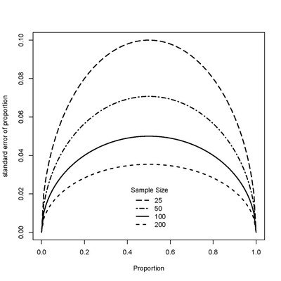
Sampling uncertainty affects the precision with which a cdf is estimated and the resultant statistics derived from the cdf such as: %-tiles (e.g., median, 25-%tile, 75-%tile, etc.).  A property of this process is that uncertainty for %-tiles is highest at the median and decreases toward zero at the extremes, 0% and 100%.  An approximation can be calculated from this formula, as usual, assuming a normal distribution:

Standard error = [p*(1-p)/n]^1/2,

Where p= proportion of interest, and n = sample size (see for example, Snedecor and Cochran 1989).  Results are illustrated in the following figure:

This figure illustrates how uncertainty of a proportion (i.e., precision) changes with both the proportion of interest and sample size.  When you look at the next “poll” in the newspaper, or magazine, you will note (usually) a statement that says the results are +/- x %; check the formula out to see how close you get to that uncertainty.  You won’t get an exact match because the pollsters use some complicated designs.

With natural resources that often display spatial structure, the combination of that spatial structure, the use of the GRTS algorithm for site selection (Stevens and Olsen, 2004), and the use of the “local variance estimator” (Stevens and Olsen, 2003) yields an unbiased estimate of precision of the cdf and derived %-tiles.  The commonly used Horwitz/Thompson variance estimator yields precision that is biased high. 

With respect to estimating the mean (e.g., abundance) or total (how many fish are in the domain), precision comes from both the uncertainty associated with the sampling process (i.e., the site selection) and the variance of the indicator of interest (across the sites sampled).  For a particular sample size (resulting in sampling uncertainty), greater precision of estimation of the mean occurs if variance is low compared with if it is high.  Given the above assumptions, the estimate will not be biased.

Up to this point, all we have been talking about are the implications of uncertainty arising from the sampling process (the site selection process) and effects onprecision, given no uncertainty in taking measurements and no temporal variation during the sampling window. 

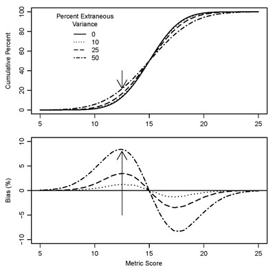
For the second part of the discussion, we’ll start again by assuming a census (so we don’t confound the illustration with sampling uncertainty) and add extraneous variance to the census picture.  Extraneous variance includes both temporal variation during the period when the sites are monitored (often called the index period) and variation associated with making the measurements (i.e., variation (or error) that arises when the same protocol is applied at nearly the same time /place, potentially with two different crews).    The effect of extraneous variance is to add noise to the resultant cdf.  The cdf generated by ourcensus with extraneous variation will be flattened compared with the cdf without extraneous variance as the following figure illustrates (modified from Kincaid, et al., 2004). 

This figure illustrates how the shape of the cdf changes with changes in extraneousvariance.  The upper figure shows how the cdf flattens with increasing extraneous variance.  The lower curve illustrates how bias in %-tiles changes depending on where you are on the cdf curve.  At the median (15 for the indicator illustrated here), no bias is introduced, indicated in the lower figure, where the curves intersect.  Bias is maximum when the cumulative Percent (proportion of interest) is about 10 (where it is biased high) or 90 (where it is biased low), illustrated in the lower curve as the maximum and minimum for each of the curves.  The arrows illustrate where the bias is maximum, at a metric score of 12.5.  The unbiased Cumulative Percent below a metric score of 12.5 is about 10.  However, added extraneous variance increases this estimate to near 20 (with 50% added extraneous variance).

Notice how the shape of the cdf creates a pinwheel as extraneous variance increases, centered on the median for a normal distribution.  Extraneousvariance does not introduce a bias in the estimate of the mean (for normal distributions), but does decrease precision of its estimate (because total variance increases).   For non-normal distributions, the bias (magnitude and direction) will depend on the shape of the cdf. 

There is a process by which the effect of extraneous variance on %-tile bias can be removed, called “deconvolution”.  See Kincaid, et al. (2004) for a detailed description of the process.  The “cost” of deconvolution is a decrease in effective sample size, and therefore on precision.  

For most real world situations, uncertainty (precision and bias) comes from both the sampling (i.e., randomization in the selection of the sample of sites) andmeasurement process.  These sources of uncertainty can be estimated (button for components of variation page), and their effects on biasand precisiondetermined and sometimes corrected.  If surveys are designed in accord with statistical principles, sampling uncertainty can be estimated. Repeated measurements during an index period allow one to estimate variation introduced by the measurement process and to make adjustments. 

This discussion assumes that the measurement process does not introduce a bias.  Clearly, if the measurement process introduces a bias, then the statistical summaries will be biased.  That bias can be confounded if bias differs across the sites.  For some purposes it might be important to estimate, and correct for, that bias; in others it might not be necessary.  In all our discussions, our context must be clear when we discuss the concepts of bias and precision: do they come from the sampling or from the measurement process?  Where do their effects introduce uncertainty in our conclusions?